Start with the numbers, because the warehouse automation breakeven lives or dies on them. A warehouse shipping two thousand orders a day employs about forty people across picking, checking, and packing. At a fully loaded cost of roughly twelve hundred dollars per person per month, that is forty-eight thousand dollars a month, or five hundred seventy-six thousand a year. That number rises every year, and a rise in the low teens over three years is unremarkable. Against it, put an automation system that covers about half that labor: purchase and implementation around four hundred thousand dollars, depreciated over five years at eighty thousand a year, plus several tens of thousands a year in maintenance and consumables. On that one line, the case looks obvious. The annual labor saving roughly covers depreciation plus maintenance. But no automation decision I have ever seen was settled on one line, because the people you save are not the same as the money you save, and the equipment costs far more than its purchase price.
Most automation projects I have watched fail died in two places. The first is counting only the equipment price and forgetting the implementation period. The second is counting heads saved and forgetting the heads you must keep. During implementation, the old process and the new system run in parallel, and training, debugging, and exception handling are all extra cost. Of the twenty people the brochure says you will save, some move into equipment maintenance, some stay to handle exceptions, and the number that actually leaves the payroll is often only sixty or seventy percent of the headline figure.
Splitting the warehouse automation breakeven into three ledgers
I split the calculation into three ledgers, because blending them guarantees an error. The first ledger is labor: the annual cost of the roles being replaced, multiplied by the realization rate you can actually achieve. The second is equipment: purchase price divided by depreciation life, plus annual maintenance, consumables, software subscriptions, and spares. The third is volatility: peak-season swings, recruiting and turnover costs, and the returns and support costs that follow error-rate changes. The third ledger is the one most business cases skip, and it is often the one that decides whether the project makes or loses money.
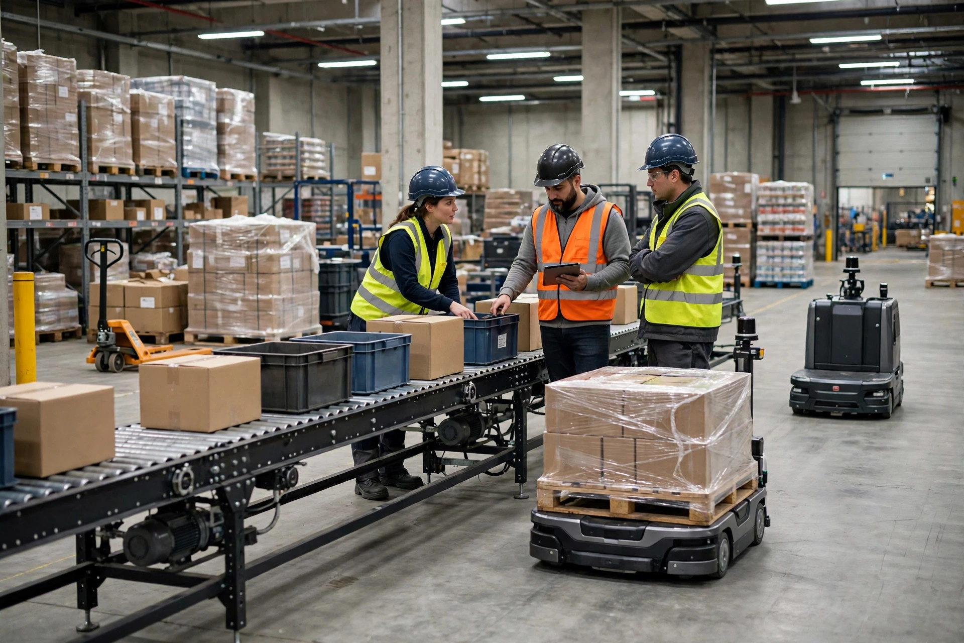
Take a consumer-goods warehouse where peak-season volume doubles. Forty people are exactly right in a normal month, but peak needs sixty, and temporary workers take a week of training before they work independently, with higher error rates than experienced staff. Automation's value here is not only heads saved; it is the peak flattened. Equipment does not resign, does not take leave, and does not need a week of peak-season training. Count only normal-month labor and the payback may look like five years. Add peak temporary labor and error costs, and payback can shorten by more than a year. The reverse is equally true: a warehouse with steady volume and a stable team that buys automation anyway will watch depreciation run faster than wage growth, and payback stretches out accordingly.
Labor costs against depreciation, year by year
| Annual cost item | Labor-only operation | Semi-automated operation | Notes |
|---|---|---|---|
| Direct labor | About $576,000 | About $340,000 | Semi-automated figure assumes forty percent realized saving |
| Equipment depreciation | Zero | About $80,000 | $400,000 spread over five years |
| Maintenance, consumables, software | Minor tool wear | About $50,000 | Includes spares and subscriptions |
| Peak temporary labor and errors | High in peak season | Materially lower | Estimated from historical peak data |
| Total | High and rising each year | Higher at first, then flattening | The breakeven is where cumulative curves cross |
The number worth watching in this table is not any single year. It is the crossing point of the cumulative curves. Year one of automation usually loses money: implementation, parallel running, and learning costs all land in year one. From year two onward, the labor-only line rises every year while the automated line flattens, and the two cumulative curves typically cross in year three or four. Talking about payback before that crossing is self-deception; only the savings after the crossing are real profit. The depreciation life you choose rewrites that crossing directly. Five years versus eight years of depreciation can shift the answer by more than a year, so the life must reflect the equipment's real working life and the vendor's support capability, not a desire to make the report look better.
Here is the counterintuitive judgment most buyers resist: the warehouse where wages are rising fastest is not always the warehouse that should automate first. If the order profile is complex, SKUs are widely dispersed, and exceptions make up a large share of orders, equipment may only cover thirty percent of the work while the remaining seventy percent still needs people. The saving ratio stays low while depreciation stays fixed, and payback gets longer, not shorter. The right first step in any warehouse automation breakeven is the most standardized work: full-case picking, standard-item sortation, fixed-route movement. Start with the slice where the numbers are cleanest.
A warehouse automation breakeven test you can actually run
To test the warehouse automation breakeven for your own site, run four steps. First, lock the replaceable scope: count the exact roles and hours in that scope, not the whole warehouse headcount. Second, set the realization rate: after transfers, retained roles, and exception handling, what share truly leaves the payroll. Third, lay out the full equipment cost: purchase, implementation, training, maintenance, consumables, software, spares, and a downtime reserve, with nothing omitted. Fourth, draw the cumulative curves: the labor-only line rising each year, the automated line at depreciation plus maintenance, and find the crossing year.
The formula itself is simple. Annual net saving equals realized labor saving minus annual depreciation minus annual maintenance cost. Payback years equal total equipment investment divided by annual net saving. Every input in that formula must have a source: labor saving from the roster, depreciation from the purchase contract and life assessment, maintenance from the vendor quotation. Any input that is roughly right makes the conclusion roughly right, and I have no patience for roughly right when a board is being asked to approve capital spending.
My decision rule is equally plain. If a conservative calculation pays back within three years, proceed. If it lands between three and five years, check whether peak-season and error benefits can pull it inside three years; if they can, proceed, and if they cannot, automate only the most standardized slice. If payback runs beyond five years, do not buy equipment yet. Standardize the process and fix rostering first, and let volume and wage growth push the breakeven toward you before spending. Automation is not better the earlier you buy it. It is profitable when the breakeven has actually arrived.
By Lao Zhou, Logistics Cost Analyst